import matplotlib.pyplot as plt
from cityseer.metrics import networks
from cityseer.tools import graphs, io![]()
Network centrality from OSM data
This notebook demonstrates how to calculate metric (shortest-path) distance centralities for a network loaded from OpenStreetMap (OSM) data. We will create a network from a buffered point, convert it into a dual graph, compute centrality measures, and visualise the results.
Prepare the network as shown in OSM examples. For example, from a relation id, bounding box, buffered point, or for extents defined from a loaded file. This example uses a buffered point.
Using a simplified representation is recommended, otherwise centrality measures will be distorted for “messier” portions of the network.
lng, lat = -0.13396079424572427, 51.51371088849723
buffer = 1500
poly_wgs, epsg_code = io.buffered_point_poly(lng, lat, buffer)
G = io.osm_graph_from_poly(poly_wgs)
G_dual = graphs.nx_to_dual(G)
INFO:cityseer.tools.graphs:Generating interpolated edge geometries.
WARNING:cityseer.tools.util:The to_crs_code parameter 4326 is not a projected CRS
INFO:cityseer.tools.io:Converting networkX graph to CRS code 32630.
WARNING:cityseer.tools.util:The to_crs_code parameter 4326 is not a projected CRS
INFO:cityseer.tools.io:Processing node x, y coordinates.
INFO:cityseer.tools.io:Processing edge geom coordinates, if present.
INFO:cityseer.tools.graphs:Removing filler nodes.
INFO:cityseer.tools.util:Creating edges STR tree.
INFO:cityseer.tools.graphs:Removing filler nodes.
INFO:cityseer.tools.graphs:Removing dangling nodes.
INFO:cityseer.tools.graphs:Removing filler nodes.
INFO:cityseer.tools.util:Creating edges STR tree.
INFO:cityseer.tools.graphs:Splitting opposing edges.
INFO:cityseer.tools.graphs:Squashing opposing nodes
INFO:cityseer.tools.graphs:Merging parallel edges within buffer of 25.
INFO:cityseer.tools.util:Creating edges STR tree.
INFO:cityseer.tools.graphs:Splitting opposing edges.
INFO:cityseer.tools.graphs:Squashing opposing nodes
INFO:cityseer.tools.graphs:Merging parallel edges within buffer of 25.
INFO:cityseer.tools.util:Creating edges STR tree.
INFO:cityseer.tools.graphs:Splitting opposing edges.
INFO:cityseer.tools.graphs:Squashing opposing nodes
INFO:cityseer.tools.graphs:Merging parallel edges within buffer of 25.
INFO:cityseer.tools.util:Creating edges STR tree.
INFO:cityseer.tools.graphs:Splitting opposing edges.
INFO:cityseer.tools.graphs:Squashing opposing nodes
INFO:cityseer.tools.graphs:Merging parallel edges within buffer of 25.
INFO:cityseer.tools.util:Creating nodes STR tree
INFO:cityseer.tools.graphs:Consolidating nodes.
INFO:cityseer.tools.graphs:Merging parallel edges within buffer of 25.
INFO:cityseer.tools.graphs:Removing filler nodes.
INFO:cityseer.tools.util:Creating nodes STR tree
INFO:cityseer.tools.graphs:Consolidating nodes.
INFO:cityseer.tools.graphs:Merging parallel edges within buffer of 25.
INFO:cityseer.tools.graphs:Removing filler nodes.
INFO:cityseer.tools.util:Creating nodes STR tree
INFO:cityseer.tools.graphs:Consolidating nodes.
INFO:cityseer.tools.graphs:Merging parallel edges within buffer of 25.
INFO:cityseer.tools.graphs:Removing filler nodes.
INFO:cityseer.tools.util:Creating nodes STR tree
INFO:cityseer.tools.graphs:Consolidating nodes.
INFO:cityseer.tools.graphs:Merging parallel edges within buffer of 25.
INFO:cityseer.tools.graphs:Removing filler nodes.
INFO:cityseer.tools.util:Creating nodes STR tree
INFO:cityseer.tools.util:Creating edges STR tree.
INFO:cityseer.tools.graphs:Snapping gapped endings.
INFO:cityseer.tools.util:Creating edges STR tree.
INFO:cityseer.tools.graphs:Splitting opposing edges.
INFO:cityseer.tools.graphs:Merging parallel edges within buffer of 25.
INFO:cityseer.tools.graphs:Removing dangling nodes.
INFO:cityseer.tools.graphs:Removing filler nodes.
INFO:cityseer.tools.util:Creating edges STR tree.
INFO:cityseer.tools.graphs:Splitting opposing edges.
INFO:cityseer.tools.graphs:Squashing opposing nodes
INFO:cityseer.tools.graphs:Merging parallel edges within buffer of 25.
INFO:cityseer.tools.util:Creating nodes STR tree
INFO:cityseer.tools.graphs:Consolidating nodes.
INFO:cityseer.tools.graphs:Merging parallel edges within buffer of 25.
INFO:cityseer.tools.graphs:Removing filler nodes.
INFO:cityseer.tools.graphs:Merging parallel edges within buffer of 50.
INFO:cityseer.tools.graphs:Ironing edges.
INFO:cityseer.tools.graphs:Merging parallel edges within buffer of 1.
INFO:cityseer.tools.graphs:Removing dangling nodes.
INFO:cityseer.tools.graphs:Removing filler nodes.
INFO:cityseer.tools.graphs:Converting graph to dual.
INFO:cityseer.tools.graphs:Preparing dual nodes
INFO:cityseer.tools.graphs:Preparing dual edges (splitting and welding geoms)Use network_structure_from_nx from the cityseer package’s io module to prepare the GeoDataFrames and NetworkStructure.
# prepare the data structures
nodes_gdf, _edges_gdf, network_structure = io.network_structure_from_nx(
    G_dual,
)
INFO:cityseer.tools.io:Preparing node and edge arrays from networkX graph.
INFO:cityseer.graph:Edge R-tree built successfully with 6904 items.Use the node_centrality_shortest function from the cityseer package’s networks module to calculate shortest metric distance centralities.
Use angular centralities with caution on automatically cleaned OSM networks, preferably only after visual inspection and manual cleaning.
distances = [500, 1000]
nodes_gdf = networks.node_centrality_shortest(
    network_structure=network_structure,
    nodes_gdf=nodes_gdf,
    distances=distances,
)
nodes_gdf.head()
INFO:cityseer.metrics.networks:Computing node centrality (shortest).
INFO:cityseer.metrics.networks: Full: 500m, 1000m| ns_node_idx | x | y | z | live | weight | primal_edge | primal_edge_node_a | primal_edge_node_b | primal_edge_idx | ... | cc_farness_500 | cc_farness_1000 | cc_harmonic_500 | cc_harmonic_1000 | cc_hillier_500 | cc_hillier_1000 | cc_betweenness_500 | cc_betweenness_1000 | cc_betweenness_beta_500 | cc_betweenness_beta_1000 | |
|---|---|---|---|---|---|---|---|---|---|---|---|---|---|---|---|---|---|---|---|---|---|
| 108285_1784656260±108286±1270370717_k0 | 0 | 698453.215258 | 5.709392e+06 | None | True | 1 | LINESTRING (698465.562 5709434.93, 698457.019 ... | 108285 | 1784656260±108286±1270370717 | 0 | ... | 6843.542690 | 68733.177822 | 0.172185 | 0.263754 | 0.131511 | 0.157362 | 0.0 | 0.0 | 0.000000 | 0.000000 |
| 25507068_9070391933_k0 | 1 | 698652.179886 | 5.709371e+06 | None | True | 1 | LINESTRING (698573.197 5709355.747, 698575.609... | 25507068 | 9070391933 | 0 | ... | 4451.295670 | 38904.140366 | 0.036087 | 0.097163 | 0.032350 | 0.083513 | 0.0 | 0.0 | 0.000000 | 0.000000 |
| 293294662_9070391933_k0 | 2 | 698664.679549 | 5.709341e+06 | None | True | 1 | LINESTRING (698577.062 5709346.311, 698581.514... | 293294662 | 9070391933 | 0 | ... | 3214.202286 | 36307.465134 | 0.027877 | 0.088749 | 0.025201 | 0.077367 | 0.0 | 0.0 | 0.000000 | 0.000000 |
| 108277_610896454_k0 | 3 | 698484.602772 | 5.709476e+06 | None | True | 1 | LINESTRING (698494.235 5709445.995, 698487.237... | 610896454 | 108277 | 0 | ... | 8397.181805 | 85174.398663 | 0.262360 | 0.377833 | 0.163031 | 0.198416 | 27.0 | 112.0 | 5.644948 | 14.987977 |
| 1784656260±108286±1270370717_610896454_k0 | 4 | 698477.371039 | 5.709448e+06 | None | True | 1 | LINESTRING (698465.562 5709434.93, 698471.303 ... | 610896454 | 1784656260±108286±1270370717 | 0 | ... | 7138.453680 | 78391.095129 | 0.265948 | 0.370422 | 0.152554 | 0.177622 | 29.0 | 29.0 | 7.648991 | 14.300224 |
5 rows × 27 columns
Exploring the results
The centrality function adds new columns to the GeoDataFrame following the naming convention cc_{centrality}_{distance}. Inspect the columns and summary statistics to understand the distribution of values.
nodes_gdf.columnsIndex(['ns_node_idx', 'x', 'y', 'z', 'live', 'weight', 'primal_edge',
'primal_edge_node_a', 'primal_edge_node_b', 'primal_edge_idx',
'dual_node', 'cc_beta_500', 'cc_beta_1000', 'cc_cycles_500',
'cc_cycles_1000', 'cc_density_500', 'cc_density_1000', 'cc_farness_500',
'cc_farness_1000', 'cc_harmonic_500', 'cc_harmonic_1000',
'cc_hillier_500', 'cc_hillier_1000', 'cc_betweenness_500',
'cc_betweenness_1000', 'cc_betweenness_beta_500',
'cc_betweenness_beta_1000'],
dtype='object')nodes_gdf["cc_hillier_500"].describe()count 2945.000000
mean 0.583945
std 0.215045
min 0.015309
25% 0.445660
50% 0.569375
75% 0.727350
max 1.132366
Name: cc_hillier_500, dtype: float64Visualising centrality
Visualise the results using the geopandas .plot() method. The first plot shows Hillier closeness at 500m and the second shows betweenness at 1000m.
fig, ax = plt.subplots(1, 1, figsize=(8, 6), facecolor="#1d1d1d")
nodes_gdf.plot(
    column="cc_hillier_500",
    cmap="magma",
    legend=False,
    ax=ax,
)
ax.axis(False)
(np.float64(697035.885372041),
np.float64(700647.6893696086),
np.float64(5709134.052703109),
np.float64(5712638.692504489))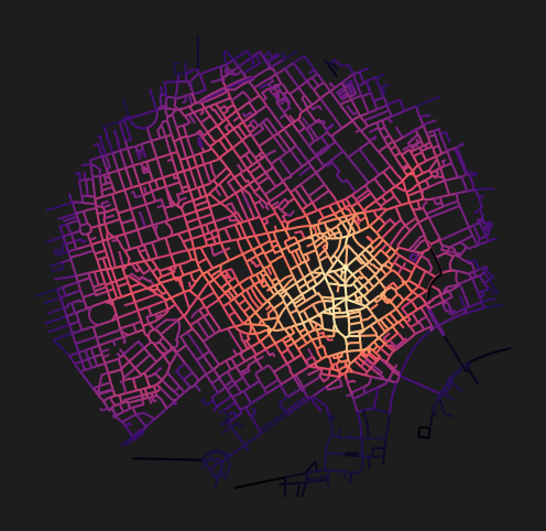
fig, ax = plt.subplots(1, 1, figsize=(8, 6), facecolor="#1d1d1d")
nodes_gdf.plot(
    column="cc_betweenness_1000",
    cmap="magma",
    legend=False,
    ax=ax,
)
ax.axis(False)
(np.float64(697035.885372041),
np.float64(700647.6893696086),
np.float64(5709134.052703109),
np.float64(5712638.692504489))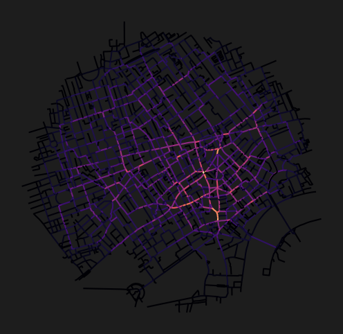
Betweenness highlights the streets that carry the most through-traffic potential. Notice how major roads and bridges tend to score highest, as they serve as critical links in the network.
Conclusion
This notebook demonstrated how to compute metric distance centralities for a network loaded directly from OpenStreetMap, using a buffered point to define the area of interest. The cleaned and simplified OSM network was converted to a dual graph, and closeness and betweenness centralities were computed and visualised at 500m and 1000m thresholds.
Next steps: To add public transport data, see GTFS Centrality. For accessibility metrics, see Accessibility.