GeoPandas

In urban analysis, working with spatial data often means handling numerous geographic features simultaneously, such as buildings, streets, or administrative boundaries. While processing each feature individually is possible, it’s considerably more efficient to manage and analyse them collectively within a structured format.

For general data analysis in Python, the pandas library is the standard tool. Pandas provides the DataFrame, a powerful table-like structure where rows represent observations (e.g., individual buildings) and columns store their attributes (e.g., height, area, land use). This structure is conceptually similar to attribute tables found in GIS software such as QGIS or ArcGIS.

GeoPandas extends pandas by incorporating first-class support for geographic data. It introduces the GeoDataFrame, which is effectively a pandas DataFrame enhanced with a dedicated column for storing geometry objects (such as points, lines, or polygons). This integration allows you to combine tabular data analysis with spatial operations.

Benefits of using GeoPandas include:

Storing geometric data alongside other attributes.
Reading and writing various spatial file formats (Shapefile, GeoPackage, GeoJSON, etc.).
Performing spatial operations (buffering, intersection, union, etc.).
Handling Coordinate Reference Systems (CRS).
Easy plotting of spatial data.

From Scratch

Although you’ll frequently load spatial data directly from files, knowing how to create a GeoDataFrame manually is beneficial. To do this, you typically need:

Tabular data (often a list of dictionaries).
Corresponding geometry objects.
A Coordinate Reference System (CRS) identifier.

Let’s begin with a simple example.

import geopandas as gpd
from shapely.geometry import Point

First, we’ll define some data as a list of dictionaries. Each dictionary will represent a city, storing its name and approximate coordinates (longitude, latitude).

data = [
    {"city": "Madrid", "x": -3.7038, "y": 40.4168},
    {"city": "Barcelona", "x": 2.1734, "y": 41.3851},
    {"city": "Valencia", "x": -0.3774, "y": 39.4699}
]

data

[{'city': 'Madrid', 'x': -3.7038, 'y': 40.4168},
 {'city': 'Barcelona', 'x': 2.1734, 'y': 41.3851},
 {'city': 'Valencia', 'x': -0.3774, 'y': 39.4699}]

Next, we need to create the corresponding geometry objects. As these are coordinates, Point objects are suitable. We can generate a list of Point objects directly from our data.

# Create Point geometries from the x and y columns
locations = []

for city in data:
    x = city["x"]
    y = city["y"]
    geom = Point(x, y)
    locations.append(geom)

locations

[<POINT (-3.704 40.417)>, <POINT (2.173 41.385)>, <POINT (-0.377 39.47)>]

With the structured data and geometry prepared, the final component is the CRS. Given that the coordinates are longitude and latitude, the appropriate CRS is WGS 84, identified by the EPSG code 4326.

We can now construct the GeoDataFrame:

gdf_cities = gpd.GeoDataFrame(
    data,  # The list of dictionaries
    geometry=locations,  # The Shapely Points
    crs=4326  # Coordinate Reference System (WGS 84)
)

gdf_cities

	city	x	y	geometry
0	Madrid	-3.7038	40.4168	POINT (-3.7038 40.4168)
1	Barcelona	2.1734	41.3851	POINT (2.1734 41.3851)
2	Valencia	-0.3774	39.4699	POINT (-0.3774 39.4699)

Indexing

Similar to pandas DataFrames, GeoDataFrames possess an index. By default, this is a range of integers. You can assign a more meaningful index using one of the columns (e.g., the city name) with the set_index() method. This often simplifies data selection.

gdf_cities = gdf_cities.set_index("city")

gdf_cities

	x	y	geometry
city
Madrid	-3.7038	40.4168	POINT (-3.7038 40.4168)
Barcelona	2.1734	41.3851	POINT (2.1734 41.3851)
Valencia	-0.3774	39.4699	POINT (-0.3774 39.4699)

You can access a row using its index. Pandas provides a special indexing method, .loc[], which allows you to access rows by their index label. This is particularly useful when you’ve set a meaningful index, such as city names.

gdf_cities.loc["Madrid"]

x                           -3.7038
y                           40.4168
geometry    POINT (-3.7038 40.4168)
Name: Madrid, dtype: object

You can also specify a column name. For instance, to retrieve the latitude of Barcelona:

gdf_cities.loc['Barcelona', "y"]

np.float64(41.3851)

To retrieve all rows for a specific column, use the : operator. For example, to get all rows for the y column:

gdf_cities.loc[:, "y"]

city
Madrid       40.4168
Barcelona    41.3851
Valencia     39.4699
Name: y, dtype: float64

An alternative way to access columns is by using the column name directly:

gdf_cities["y"]

city
Madrid       40.4168
Barcelona    41.3851
Valencia     39.4699
Name: y, dtype: float64

A particularly powerful feature of GeoDataFrames is the ability to filter rows based on their properties. To do this, you create a boolean mask, which can then be used to exclude rows you are not interested in. For instance, if you want to filter the cities to include only those with a latitude greater than 40, you can proceed as follows:

# Create a boolean mask
mask = gdf_cities["y"] > 40

mask

city
Madrid        True
Barcelona     True
Valencia     False
Name: y, dtype: bool

This mask is a pandas Series of boolean values, where True indicates that the condition (y > 40) is met, and False indicates it is not. You can now apply this mask to filter the rows in the original GeoDataFrame.

# Use the mask to filter the rows
gdf_cities.loc[mask]

	x	y	geometry
city
Madrid	-3.7038	40.4168	POINT (-3.7038 40.4168)
Barcelona	2.1734	41.3851	POINT (2.1734 41.3851)

As shown, only two rows are returned because Valencia, the third city, has a latitude below 40.

Geospatial

GeoDataFrames possess special properties stemming from their spatial nature.

GeoPandas formally designates a particular column as the geometry; this is typically done during the creation of the GeoDataFrame. The geometry column contains Shapely geometry objects, which can be points, lines, or polygons. This column is often called geometry, but this is not always the case.

gdf_cities.geometry

city
Madrid       POINT (-3.7038 40.4168)
Barcelona     POINT (2.1734 41.3851)
Valencia     POINT (-0.3774 39.4699)
Name: geometry, dtype: geometry

Similarly, GeoPandas formally associates the geometry with a given CRS, accessible via the .crs attribute.

gdf_cities.crs

<Geographic 2D CRS: EPSG:4326>
Name: WGS 84
Axis Info [ellipsoidal]:
- Lat[north]: Geodetic latitude (degree)
- Lon[east]: Geodetic longitude (degree)
Area of Use:
- name: World.
- bounds: (-180.0, -90.0, 180.0, 90.0)
Datum: World Geodetic System 1984 ensemble
- Ellipsoid: WGS 84
- Prime Meridian: Greenwich

GeoPandas conveniently integrates with matplotlib for straightforward plotting. Calling .plot() on a GeoDataFrame will render its geometries.

gdf_cities.plot()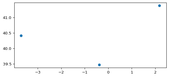

Coordinate Transformations

GeoPandas makes CRS transformation very easy with the to_crs() method. Ensure you use a projected coordinate reference system when performing detailed spatial analysis. Let’s convert our cities GeoDataFrame to EPSG:3035, a projected equal-area CRS suitable for Europe (ETRS89-LAEA).

gdf_cities_proj = gdf_cities.to_crs(3035)

gdf_cities_proj

	x	y	geometry
city
Madrid	-3.7038	40.4168	POINT (3159390.356 2029850.92)
Barcelona	2.1734	41.3851	POINT (3664996.992 2065549.826)
Valencia	-0.3774	39.4699	POINT (3426003.188 1881060.49)

Notice how the x and y columns no longer match the geometry, as the geometry is now in metres according to EPSG:3035. The .crs attribute reflects this change:

gdf_cities_proj.crs

<Projected CRS: EPSG:3035>
Name: ETRS89-extended / LAEA Europe
Axis Info [cartesian]:
- Y[north]: Northing (metre)
- X[east]: Easting (metre)
Area of Use:
- name: Europe - European Union (EU) countries and candidates. Europe - onshore and offshore: Albania; Andorra; Austria; Belgium; Bosnia and Herzegovina; Bulgaria; Croatia; Cyprus; Czechia; Denmark; Estonia; Faroe Islands; Finland; France; Germany; Gibraltar; Greece; Hungary; Iceland; Ireland; Italy; Kosovo; Latvia; Liechtenstein; Lithuania; Luxembourg; Malta; Monaco; Montenegro; Netherlands; North Macedonia; Norway including Svalbard and Jan Mayen; Poland; Portugal including Madeira and Azores; Romania; San Marino; Serbia; Slovakia; Slovenia; Spain including Canary Islands; Sweden; Switzerland; Türkiye (Turkey); United Kingdom (UK) including Channel Islands and Isle of Man; Vatican City State.
- bounds: (-35.58, 24.6, 44.83, 84.73)
Coordinate Operation:
- name: Europe Equal Area 2001
- method: Lambert Azimuthal Equal Area
Datum: European Terrestrial Reference System 1989 ensemble
- Ellipsoid: GRS 1980
- Prime Meridian: Greenwich

Plotting the transformed data shows the locations relative to the new projected coordinate system.

gdf_cities_proj.plot()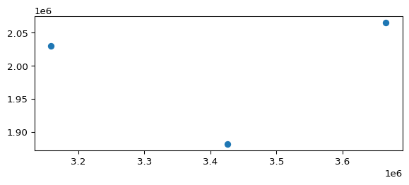

Spatial Operations

GeoPandas enables you to apply spatial operations directly to GeoDataFrames or GeoSeries. These operations are applied element-wise.

For instance, to create a 100km buffer around each city:

# The buffer distance is in the units of the CRS (metres for EPSG:3035)
gdf_cities_proj["geometry"] = gdf_cities_proj.geometry.buffer(100000)  # 100km buffer

gdf_cities_proj.plot()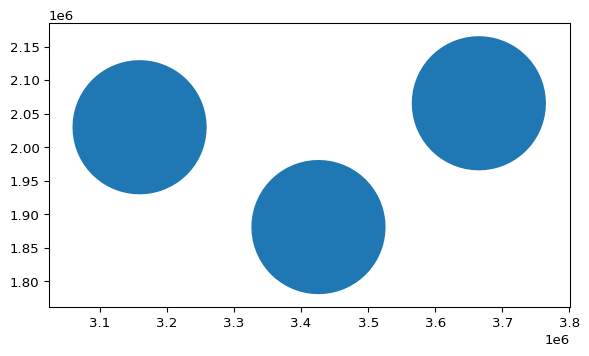

Alternatively, you can calculate the distance from each feature in a GeoDataFrame to a single Shapely geometry object. Let’s determine the distance from each city buffer to a specific point (also defined in EPSG:3035 coordinates):

# Define a point in the same CRS (EPSG:3035)
pt = Point(3300000, 2000000)

# Calculate distance from each geometry in the GeoSeries to the point
gdf_cities_proj.geometry.distance(pt)

city
Madrid        43770.428827
Barcelona    270860.150569
Valencia      73357.551677
dtype: float64

Creating and Updating Columns

If we wished to create a new column named ‘easting’ and assign it the x-coordinate of the geometry, we could proceed as follows:

gdf_cities_proj['easting'] = gdf_cities_proj.geometry.centroid.x

gdf_cities_proj

	x	y	geometry	easting
city
Madrid	-3.7038	40.4168	POLYGON ((3259390.356 2029850.92, 3258908.829 ...	3.159390e+06
Barcelona	2.1734	41.3851	POLYGON ((3764996.992 2065549.826, 3764515.465...	3.664997e+06
Valencia	-0.3774	39.4699	POLYGON ((3526003.188 1881060.49, 3525521.661 ...	3.426003e+06

Each geometry row in the DataFrame is a Shapely geometry, so you can use standard Shapely syntax to access properties such as the centroid or its x-coordinate.

If you decide instead to update the existing x and y columns, you can reference them directly:

gdf_cities_proj['x'] = gdf_cities_proj.geometry.centroid.x
gdf_cities_proj['y'] = gdf_cities_proj.geometry.centroid.y

gdf_cities_proj

	x	y	geometry	easting
city
Madrid	3.159390e+06	2.029851e+06	POLYGON ((3259390.356 2029850.92, 3258908.829 ...	3.159390e+06
Barcelona	3.664997e+06	2.065550e+06	POLYGON ((3764996.992 2065549.826, 3764515.465...	3.664997e+06
Valencia	3.426003e+06	1.881060e+06	POLYGON ((3526003.188 1881060.49, 3525521.661 ...	3.426003e+06

DataFrames offer an extensive variety of useful methods; here, we will use the drop method to remove the column we no longer wish to retain:

gdf_cities_proj = gdf_cities_proj.drop(columns=['easting'])

gdf_cities_proj

	x	y	geometry
city
Madrid	3.159390e+06	2.029851e+06	POLYGON ((3259390.356 2029850.92, 3258908.829 ...
Barcelona	3.664997e+06	2.065550e+06	POLYGON ((3764996.992 2065549.826, 3764515.465...
Valencia	3.426003e+06	1.881060e+06	POLYGON ((3526003.188 1881060.49, 3525521.661 ...

Working with Data

Reading Data

GeoPandas can read various spatial data formats, such as Shapefiles, GeoPackages, and GeoJSON files. The read_file() function is the primary method for this. Note that the file path in the example below must be adjusted to point to the actual location of the file on your computer.

mad_bldgs = gpd.read_file('../data/madrid_buildings/madrid_bldgs.gpkg')

mad_bldgs.head()

	mean_height	area	perimeter	compactness	orientation	volume	floor_area_ratio	form_factor	corners	shape_index	fractal_dimension	geometry
0	NaN	187.418714	58.669276	0.491102	40.235999	NaN	NaN	NaN	4	0.700787	1.026350	POLYGON ((448688.642 4492911, 448678.351 44928...
1	7.0	39.082821	26.992208	0.472874	10.252128	273.579749	78.165643	5.410857	4	0.687658	1.041691	POLYGON ((440862.665 4482604.017, 440862.64 44...
2	7.0	39.373412	27.050303	0.475086	10.252128	275.613883	78.746824	5.400665	4	0.689265	1.040760	POLYGON ((440862.681 4482608.269, 440862.665 4...
3	7.5	37.933979	26.739878	0.464266	10.252129	284.504846	75.867959	5.513124	4	0.681371	1.045072	POLYGON ((440862.705 4482612.365, 440862.681 4...
4	7.0	39.013701	26.972641	0.472468	10.183618	273.095907	78.027402	5.412350	4	0.687363	1.041798	POLYGON ((440880.29 4482607.963, 440880.274 44...

The head() method shows the first few rows of the GeoDataFrame, including the geometry column. The CRS is automatically detected and set.

Plotting

Let’s plot the data.

mad_bldgs.plot()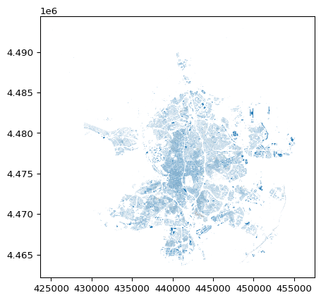

To zoom in when plotting, you can set your x and y-axis limits. For a cleaner plot, it is also generally preferable to turn off the axes so that the coordinates do not render.

ax = mad_bldgs.plot()

ax.set_xlim(439000, 442000)
ax.set_ylim(4473000, 4476000)
ax.axis('off')

(np.float64(439000.0),
 np.float64(442000.0),
 np.float64(4473000.0),
 np.float64(4476000.0))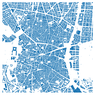

Let’s create a new column named area, which we will set to the value of each geometry’s area. Then, we will plot the data again, this time rendering the colour according to the building’s area.

mad_bldgs['area'] = mad_bldgs.geometry.area

ax = mad_bldgs.plot(
    column='area',
    cmap='viridis',
    vmax=10000,
)

ax.set_xlim(439000, 442000)
ax.set_ylim(4473000, 4476000)
ax.axis('off')

(np.float64(439000.0),
 np.float64(442000.0),
 np.float64(4473000.0),
 np.float64(4476000.0))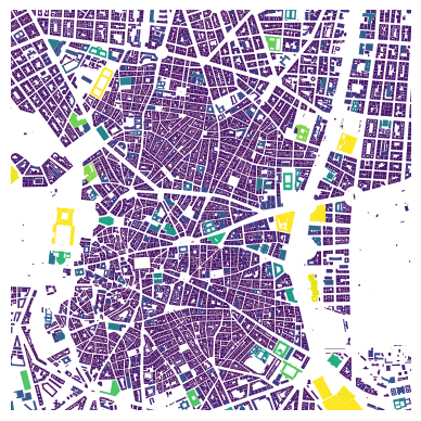

Saving Data

GeoPandas can save GeoDataFrames to various formats, including Shapefiles, GeoPackages, and GeoJSON files. The to_file() method is used for this purpose. You can specify the format using the driver parameter.

mad_bldgs.to_file('bldgs_w_area.gpkg', driver='GPKG')