Download geospatial features from OpenStreetMap using osmnx
Prepare and clean downloaded data for analysis
Calculate urban morphology metrics with momepy
Export analysis results to spatial data files
Building upon our previous explorations of Python, Shapely, and GeoPandas, this lesson introduces the broader Python geospatial ecosystem. We will focus on two particularly useful libraries: osmnx for acquiring urban data from OpenStreetMap, and momepy for conducting urban morphological analysis.
Prerequisites and Setup
Ensure you have osmnx and momepy installed in your Python environment. If you are following along with a notebook, you can install these using pip.
# Use an exclamation mark to run in notebooks!pip install osmnx momepy
Packages such as matplotlib and geopandas are often already installed by default but, if necessary, you can install them in the same way.
Importing Libraries
Let’s import the necessary packages:
import geopandas as gpd# use an alias for convenienceimport osmnx as oximport momepyimport matplotlib.pyplot as plt
/home/runner/work/cityseer-examples/cityseer-examples/.venv/lib/python3.12/site-packages/tqdm/auto.py:21: TqdmWarning: IProgress not found. Please update jupyter and ipywidgets. See https://ipywidgets.readthedocs.io/en/stable/user_install.html
  from .autonotebook import tqdm as notebook_tqdm
osmnx
osmnx is a Python package that simplifies downloading and working with geospatial data from OpenStreetMap (OSM), such as building footprints or points of interest.
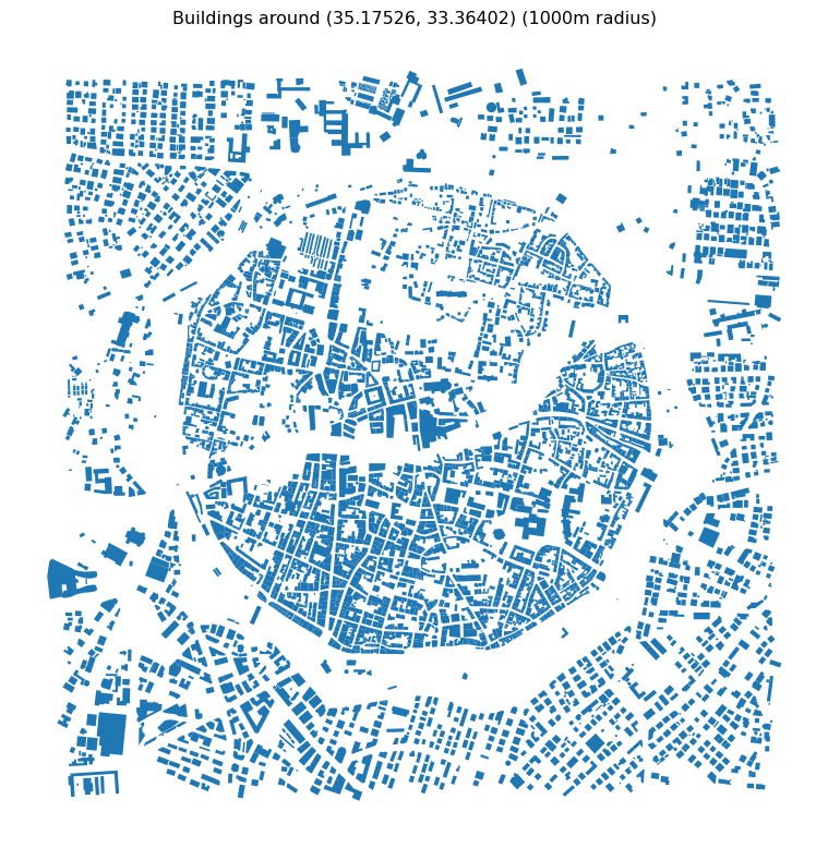
This example demonstrates how to download building footprints within a 1km radius of a specified location in Nicosia, Cyprus, defined by its coordinates. osmnx provides several methods for downloading data; here, we will use features_from_point.
# Define the point of interest (latitude, longitude) and distancecenter_point = (35.17526, 33.36402)distance_m =1000# Download building footprintsgdf_buildings = ox.features_from_point( center_point, tags={"building": True}, dist=distance_m)
osmnx returns GeoDataFrames which, as shown in the previous lesson, are ideal for spatial analysis in Python. Note the tags={"building": True} argument, which instructs osmnx to fetch all features tagged as buildings in OSM. By changing these tags, you can also download other types of features, such as roads or parks.
It is good practice to inspect the data you have downloaded. The head() function displays the first few rows of the GeoDataFrame, allowing you to quickly check the data structure and attributes.
# Display the first few rows of the buildings GeoDataFramegdf_buildings.head()
geometry
amenity
building
bus
name
public_transport
addr:city
addr:housenumber
addr:postcode
addr:street
...
association
house
attraction
species:wikidata
species:wikipedia
drinking_water
fountain
fixme
type
inscription
element
id
node
4338033483
POINT (33.36625 35.18368)
bus_station
yes
yes
İtimat (Lefkoşa Mağusa Servis)
station
NaN
NaN
NaN
NaN
...
NaN
NaN
NaN
NaN
NaN
NaN
NaN
NaN
NaN
NaN
5206675859
POINT (33.35992 35.17344)
NaN
yes
NaN
NaN
NaN
NaN
NaN
NaN
NaN
...
NaN
NaN
NaN
NaN
NaN
NaN
NaN
NaN
NaN
NaN
12027040593
POINT (33.35773 35.17435)
NaN
yes
NaN
Apostolic Nunciature to Cyprus
NaN
Nicosia
1
1010
Pafou
...
NaN
NaN
NaN
NaN
NaN
NaN
NaN
NaN
NaN
NaN
relation
2580980
POLYGON ((33.36224 35.17641, 33.3628 35.17652,...
NaN
yes
NaN
Büyük Han
NaN
NaN
NaN
NaN
NaN
...
NaN
NaN
NaN
NaN
NaN
NaN
NaN
NaN
multipolygon
OTTOMAN
2785751
POLYGON ((33.36028 35.17739, 33.36019 35.17701...
NaN
yes
NaN
NaN
NaN
NaN
NaN
NaN
Müftü Raci Sokak
...
NaN
NaN
NaN
NaN
NaN
NaN
NaN
NaN
multipolygon
NaN
5 rows × 185 columns
You can also plot the downloaded data:
# Set up a plotfig, ax = plt.subplots(figsize=(10, 10))# Plot the buildingsgdf_buildings.plot(ax=ax)# Set the title and remove the axis for a cleaner lookax.set_title(f"Buildings around {center_point} ({distance_m}m radius)")ax.axis("off")
For more detailed information on different ways to query OSM features data, refer to the osmnxfeatures documentation.
Data Preparation
To streamline the subsequent analysis, it is advisable to first filter for the types of geometry you intend to work with. In this instance, we are interested in polygon or multi-polygon geometries and will discard other types, such as points or linestrings.
# Filter out non-polygon geometriesgdf_buildings = gdf_buildings[ gdf_buildings.geometry.type.isin(['Polygon', 'MultiPolygon'])]gdf_buildings.head()
geometry
amenity
building
bus
name
public_transport
addr:city
addr:housenumber
addr:postcode
addr:street
...
association
house
attraction
species:wikidata
species:wikipedia
drinking_water
fountain
fixme
type
inscription
element
id
relation
2580980
POLYGON ((33.36224 35.17641, 33.3628 35.17652,...
NaN
yes
NaN
Büyük Han
NaN
NaN
NaN
NaN
NaN
...
NaN
NaN
NaN
NaN
NaN
NaN
NaN
NaN
multipolygon
OTTOMAN
2785751
POLYGON ((33.36028 35.17739, 33.36019 35.17701...
NaN
yes
NaN
NaN
NaN
NaN
NaN
NaN
Müftü Raci Sokak
...
NaN
NaN
NaN
NaN
NaN
NaN
NaN
NaN
multipolygon
NaN
3403727
POLYGON ((33.36277 35.17718, 33.36274 35.17688...
NaN
yes
NaN
Kumarcılar Hanı
NaN
NaN
NaN
NaN
NaN
...
NaN
NaN
NaN
NaN
NaN
NaN
NaN
NaN
multipolygon
NaN
8756098
POLYGON ((33.36483 35.17161, 33.36483 35.17161...
NaN
yes
NaN
NaN
NaN
NaN
NaN
NaN
NaN
...
NaN
NaN
NaN
NaN
NaN
NaN
NaN
NaN
multipolygon
NaN
8762332
POLYGON ((33.36003 35.17852, 33.36002 35.17849...
NaN
house
NaN
NaN
NaN
NaN
NaN
NaN
NaN
...
NaN
NaN
NaN
NaN
NaN
NaN
NaN
NaN
multipolygon
NaN
5 rows × 185 columns
Secondly, we will reset the index so that all features are neatly indexed from zero upwards, without duplicates.
# Reset the indexgdf_buildings = gdf_buildings.reset_index(drop=True)gdf_buildings.head()
geometry
amenity
building
bus
name
public_transport
addr:city
addr:housenumber
addr:postcode
addr:street
...
association
house
attraction
species:wikidata
species:wikipedia
drinking_water
fountain
fixme
type
inscription
0
POLYGON ((33.36224 35.17641, 33.3628 35.17652,...
NaN
yes
NaN
Büyük Han
NaN
NaN
NaN
NaN
NaN
...
NaN
NaN
NaN
NaN
NaN
NaN
NaN
NaN
multipolygon
OTTOMAN
1
POLYGON ((33.36028 35.17739, 33.36019 35.17701...
NaN
yes
NaN
NaN
NaN
NaN
NaN
NaN
Müftü Raci Sokak
...
NaN
NaN
NaN
NaN
NaN
NaN
NaN
NaN
multipolygon
NaN
2
POLYGON ((33.36277 35.17718, 33.36274 35.17688...
NaN
yes
NaN
Kumarcılar Hanı
NaN
NaN
NaN
NaN
NaN
...
NaN
NaN
NaN
NaN
NaN
NaN
NaN
NaN
multipolygon
NaN
3
POLYGON ((33.36483 35.17161, 33.36483 35.17161...
NaN
yes
NaN
NaN
NaN
NaN
NaN
NaN
NaN
...
NaN
NaN
NaN
NaN
NaN
NaN
NaN
NaN
multipolygon
NaN
4
POLYGON ((33.36003 35.17852, 33.36002 35.17849...
NaN
house
NaN
NaN
NaN
NaN
NaN
NaN
NaN
...
NaN
NaN
NaN
NaN
NaN
NaN
NaN
NaN
multipolygon
NaN
5 rows × 185 columns
Thirdly, we will drop any columns not relevant to our analysis. In this case, we will retain the geometry column and the building column.
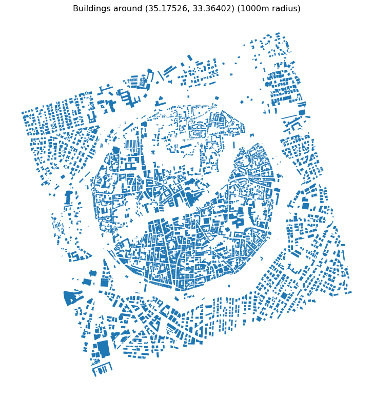
Before performing morphological analysis, it is necessary to ensure your data is in a projected Coordinate Reference System (CRS). Morphological metrics often involve measurements of distance and area, which are only accurate in a projected CRS. For Nicosia, we will use EPSG:3035 (ETRS89 / LAEA Europe), a European projection.
# Set the target CRSgdf_buildings_proj = gdf_buildings.to_crs(3035)
Let’s replot the building data to ensure everything is in order.
# Set up a plotfig, ax = plt.subplots(figsize=(10, 10))# Plot the buildingsgdf_buildings_proj.plot(ax=ax)# Set the title and remove axisax.set_title(f"Buildings around {center_point} ({distance_m}m radius)")ax.axis("off")
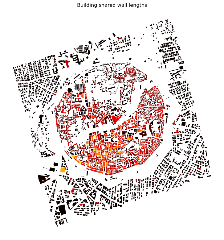
momepy is a library for the quantitative analysis of urban form – also known as urban morphology. It operates primarily on GeoDataFrames and provides a range of functions for calculating various morphological metrics.
By way of example, we will explore two of these functions.
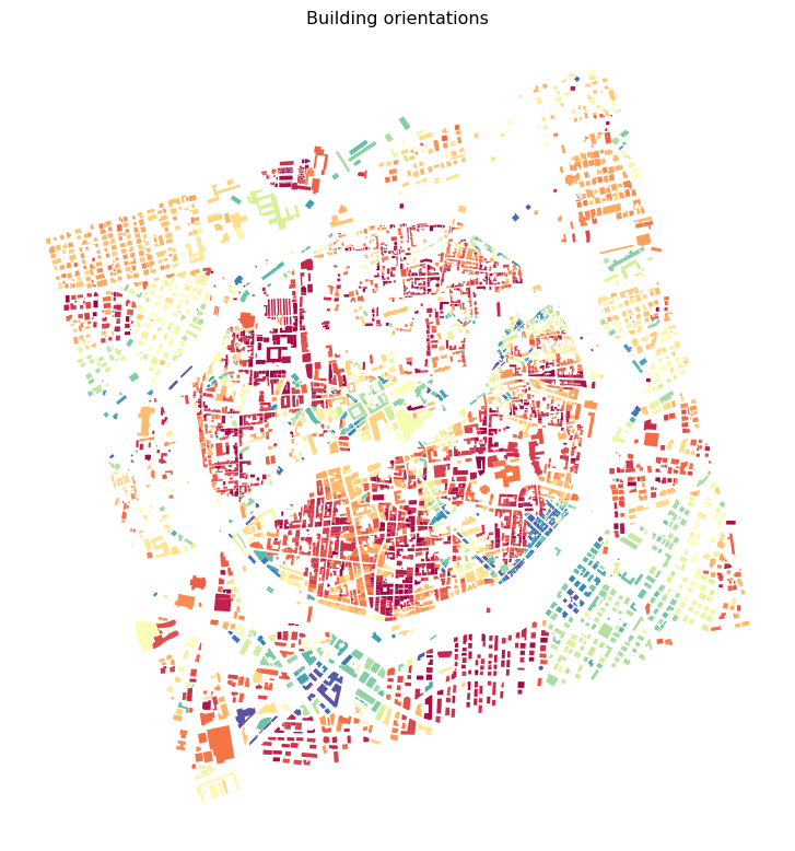
Building Orientations
momepy can calculate the orientation of building footprints using the orientation function.
Many other functions are available in momepy for calculating various morphological metrics. For a comprehensive list, please refer to the momepy documentation.
Exercises
Use osmnx to download a different feature type (e.g., parks with tags={"leisure": "park"}) for the same area. Plot the result.
Explore the momepy documentation and calculate a different morphological metric (e.g., momepy.elongation or momepy.circular_compactness) on the building footprints. What do the values tell you about building shapes?
Download building footprints for a location of your choice (a different city or neighbourhood). Compare building orientations between the two areas.
Summary
This has been a brief exploration of the broader Python geospatial ecosystem, focusing on osmnx for downloading urban data from OpenStreetMap and momepy for conducting urban morphology analysis. This is just a small sample of what these and other tools can achieve.
Remember that with GeoPandas, you can export your data. So, after downloading data and running any variety of metrics using available Python packages, you can then export the file, which can be further visualised or manipulated with packages such as QGIS. For example, you can export your data to a GeoPackage file using the to_file method:
Next: Data Science introduces dimensionality reduction and prediction with scikit-learn. The osmnx skills from this chapter are used in many of the Cityseer Recipes, particularly the Network Preparation examples.