Open In Colab

Metric distance network centrality

Calculate metric distance centralities from a geopandas GeoDataFrame.

import geopandas as gpd
import matplotlib.pyplot as plt
from cityseer.metrics import networks
from cityseer.tools import graphs, io

Prepare the network as shown in other examples. Working with the dual graph is recommended.

streets_gpd = gpd.read_file("data/madrid_streets/street_network.gpkg")
streets_gpd = streets_gpd.explode(reset_index=True)
G = io.nx_from_generic_geopandas(streets_gpd)

INFO:cityseer.tools.graphs:Merging parallel edges within buffer of 1.

Load the study area boundary and set live=True for nodes inside the boundary. Nodes outside the boundary act as a buffer to prevent edge rolloff — they are used for routing but metrics are not computed for them. See the live nodes example for more details.

from shapely import geometry

bounds_gpd = gpd.read_file("data/madrid_bounds/madrid_bounds.gpkg")
boundary_poly = bounds_gpd.geometry.iloc[0]
for node_idx, node_data in G.nodes(data=True):
    node_pnt = geometry.Point(node_data["x"], node_data["y"])
    if node_pnt.intersects(boundary_poly):
        G.nodes[node_idx]["live"] = True
    else:
        G.nodes[node_idx]["live"] = False

G_dual = graphs.nx_to_dual(G)

INFO:cityseer.tools.graphs:Converting graph to dual.
INFO:cityseer.tools.graphs:Preparing dual nodes
INFO:cityseer.tools.graphs:Preparing dual edges (splitting and welding geoms)

Use network_structure_from_nx from the cityseer package’s io module to prepare the GeoDataFrames and NetworkStructure.

# prepare the data structures
nodes_gdf, _edges_gdf, network_structure = io.network_structure_from_nx(
    G_dual,
)

INFO:cityseer.tools.io:Preparing node and edge arrays from networkX graph.
INFO:cityseer.graph:Edge R-tree built successfully with 452252 items.

Use the node_centrality_shortest function from the cityseer package’s networks module to calculate shortest metric distance centralities. The function requires a NetworkStructure and nodes GeoDataFrame prepared with the network_structure_from_nx function in the previous step.

The function can calculate centralities for numerous distances at once via the distances parameter, which accepts a list of distances.

The function returns the nodes GeoDataFrame with the outputs of the centralities added as columns. The columns are named cc_{centrality}_{distance}. Standard geopandas functionality can be used to explore, visualise, or save the results. See the documentation for more information on the available centrality formulations.

distances = [500, 2000]
nodes_gdf = networks.node_centrality_shortest(
    network_structure=network_structure,
    nodes_gdf=nodes_gdf,
    distances=distances,
)
nodes_gdf.head()

INFO:cityseer.metrics.networks:Computing node centrality (shortest).
INFO:cityseer.metrics.networks:  Full: 500m, 2000m

	ns_node_idx	x	y	z	live	weight	primal_edge	primal_edge_node_a	primal_edge_node_b	...	cc_hillier_500	cc_hillier_2000
x429937.0-y4446780.0_x429947.0-y4446831.0_k0	0	429942.000000	4.446806e+06	None	False	1	LINESTRING (429937 4446780, 429947 4446831)	x429937.0-y4446780.0	x429947.0-y4446831.0	...	NaN	NaN
x429804.0-y4446863.0_x429937.0-y4446780.0_k0	1	429869.198345	4.446814e+06	None	False	1	LINESTRING (429804 4446863, 429921 4446775, 42...	x429937.0-y4446780.0	x429804.0-y4446863.0	...	NaN	NaN
x429804.0-y4446863.0_x429947.0-y4446831.0_k0	2	429875.500000	4.446847e+06	None	False	1	LINESTRING (429804 4446863, 429947 4446831)	x429947.0-y4446831.0	x429804.0-y4446863.0	...	NaN	NaN
x429947.0-y4446831.0_x429960.0-y4446891.0_k0	3	429953.500000	4.446861e+06	None	False	1	LINESTRING (429947 4446831, 429960 4446891)	x429947.0-y4446831.0	x429960.0-y4446891.0	...	NaN	NaN
x429804.0-y4446863.0_x429815.0-y4446919.0_k0	4	429809.500000	4.446891e+06	None	False	1	LINESTRING (429804 4446863, 429815 4446919)	x429804.0-y4446863.0	x429815.0-y4446919.0	...	NaN	NaN

5 rows × 27 columns

nodes_gdf.columns

Index(['ns_node_idx', 'x', 'y', 'z', 'live', 'weight', 'primal_edge',
       'primal_edge_node_a', 'primal_edge_node_b', 'primal_edge_idx',
       'dual_node', 'cc_beta_500', 'cc_beta_2000', 'cc_cycles_500',
       'cc_cycles_2000', 'cc_density_500', 'cc_density_2000', 'cc_farness_500',
       'cc_farness_2000', 'cc_harmonic_500', 'cc_harmonic_2000',
       'cc_hillier_500', 'cc_hillier_2000', 'cc_betweenness_500',
       'cc_betweenness_2000', 'cc_betweenness_beta_500',
       'cc_betweenness_beta_2000'],
      dtype='object')

nodes_gdf["cc_betweenness_2000"].describe()

count    220036.000000
mean       4112.003420
std       13060.583547
min           0.000000
25%           0.000000
50%           0.000000
75%         343.000000
max      244674.750000
Name: cc_betweenness_2000, dtype: float64

fig, ax = plt.subplots(1, 1, figsize=(8, 6), facecolor="#1d1d1d")
nodes_gdf.plot(
    column="cc_harmonic_500",
    cmap="magma",
    legend=False,
    ax=ax,
)
ax.set_xlim(438500, 438500 + 3500)
ax.set_ylim(4472500, 4472500 + 3500)
ax.axis(False)

(np.float64(438500.0),
 np.float64(442000.0),
 np.float64(4472500.0),
 np.float64(4476000.0))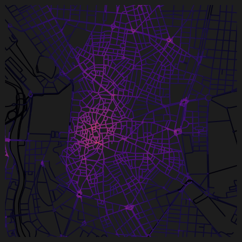

fig, ax = plt.subplots(1, 1, figsize=(8, 6), facecolor="#1d1d1d")
nodes_gdf.plot(
    column="cc_betweenness_2000",
    cmap="magma",
    legend=False,
    ax=ax,
)
ax.set_xlim(438500, 438500 + 3500)
ax.set_ylim(4472500, 4472500 + 3500)
ax.axis(False)

(np.float64(438500.0),
 np.float64(442000.0),
 np.float64(4472500.0),
 np.float64(4476000.0))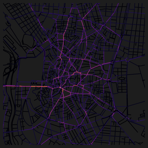

Alternatively, you can define the distance thresholds using a list of minutes instead.

nodes_gdf = networks.node_centrality_shortest(
    network_structure=network_structure,
    nodes_gdf=nodes_gdf,
    minutes=[15],
)

INFO:cityseer.metrics.networks:Computing node centrality (shortest).
INFO:cityseer.metrics.networks:  Full: 1200m

The function will map the minutes values into the equivalent distances, which are reported in the logged output.

nodes_gdf.columns

Index(['ns_node_idx', 'x', 'y', 'z', 'live', 'weight', 'primal_edge',
       'primal_edge_node_a', 'primal_edge_node_b', 'primal_edge_idx',
       'dual_node', 'cc_beta_500', 'cc_beta_2000', 'cc_cycles_500',
       'cc_cycles_2000', 'cc_density_500', 'cc_density_2000', 'cc_farness_500',
       'cc_farness_2000', 'cc_harmonic_500', 'cc_harmonic_2000',
       'cc_hillier_500', 'cc_hillier_2000', 'cc_betweenness_500',
       'cc_betweenness_2000', 'cc_betweenness_beta_500',
       'cc_betweenness_beta_2000', 'cc_beta_1200', 'cc_cycles_1200',
       'cc_density_1200', 'cc_farness_1200', 'cc_harmonic_1200',
       'cc_hillier_1200', 'cc_betweenness_1200', 'cc_betweenness_beta_1200'],
      dtype='object')

As per the function logging outputs, 15 minutes has been mapped to 1200m at default speed_m_s, so the corresponding outputs can be visualised using the 1200m columns. Use the configurable speed_m_s parameter to set a custom metres per second walking speed.

fig, ax = plt.subplots(1, 1, figsize=(8, 6), facecolor="#1d1d1d")
nodes_gdf.plot(
    column="cc_harmonic_1200",
    cmap="magma",
    legend=False,
    ax=ax,
)
ax.set_xlim(438500, 438500 + 3500)
ax.set_ylim(4472500, 4472500 + 3500)
ax.axis(False)

(np.float64(438500.0),
 np.float64(442000.0),
 np.float64(4472500.0),
 np.float64(4476000.0))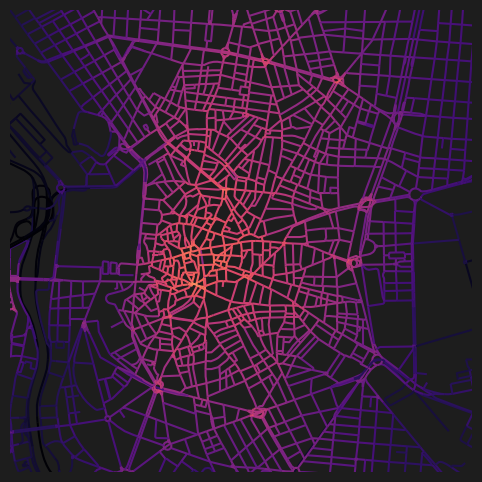

For spatial-impedance weighted forms of centralities (beta variants), you can specify the beta parameter explicitly. These will otherwise be extrapolated automatically from the distances or minutes parameters. See the documentation for more information on how spatial impedances are converted to distance thresholds.

nodes_gdf = networks.node_centrality_shortest(
    network_structure=network_structure,
    nodes_gdf=nodes_gdf,
    betas=[0.01],
)

INFO:cityseer.metrics.networks:Computing node centrality (shortest).
INFO:cityseer.metrics.networks:  Full: 400m

nodes_gdf.columns

Index(['ns_node_idx', 'x', 'y', 'z', 'live', 'weight', 'primal_edge',
       'primal_edge_node_a', 'primal_edge_node_b', 'primal_edge_idx',
       'dual_node', 'cc_beta_500', 'cc_beta_2000', 'cc_cycles_500',
       'cc_cycles_2000', 'cc_density_500', 'cc_density_2000', 'cc_farness_500',
       'cc_farness_2000', 'cc_harmonic_500', 'cc_harmonic_2000',
       'cc_hillier_500', 'cc_hillier_2000', 'cc_betweenness_500',
       'cc_betweenness_2000', 'cc_betweenness_beta_500',
       'cc_betweenness_beta_2000', 'cc_beta_1200', 'cc_cycles_1200',
       'cc_density_1200', 'cc_farness_1200', 'cc_harmonic_1200',
       'cc_hillier_1200', 'cc_betweenness_1200', 'cc_betweenness_beta_1200',
       'cc_beta_400', 'cc_cycles_400', 'cc_density_400', 'cc_farness_400',
       'cc_harmonic_400', 'cc_hillier_400', 'cc_betweenness_400',
       'cc_betweenness_beta_400'],
      dtype='object')

fig, ax = plt.subplots(1, 1, figsize=(8, 6), facecolor="#1d1d1d")
nodes_gdf.plot(
    column="cc_beta_400",
    cmap="magma",
    legend=False,
    ax=ax,
)
ax.set_xlim(438500, 438500 + 3500)
ax.set_ylim(4472500, 4472500 + 3500)
ax.axis(False)

(np.float64(438500.0),
 np.float64(442000.0),
 np.float64(4472500.0),
 np.float64(4476000.0))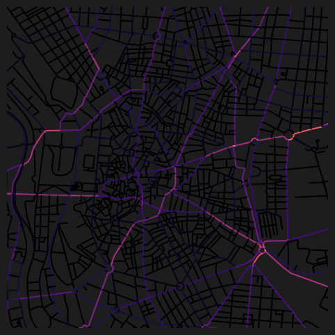

Sampled centrality for larger distances

For larger distance thresholds, the computational cost increases substantially. The node_centrality_shortest function supports a sample=True parameter that uses a sampling strategy to compute centralities more efficiently at larger scales while maintaining a relatively high degree of rank performance. Rather use non-sampled when generating publication-quality results.

distances = [500, 10000]
nodes_gdf = networks.node_centrality_shortest(
    network_structure=network_structure,
    nodes_gdf=nodes_gdf,
    distances=distances,
    sample=True,
)
nodes_gdf.columns

INFO:cityseer.metrics.networks:Computing node centrality (shortest).
WARNING:cityseer.metrics.networks:Sampling is experimental: API and behaviour may change in future releases.
INFO:cityseer.metrics.networks:  Full: 500m
INFO:cityseer.metrics.networks:  Sampled 10000m: p=17%

Index(['ns_node_idx', 'x', 'y', 'z', 'live', 'weight', 'primal_edge',
       'primal_edge_node_a', 'primal_edge_node_b', 'primal_edge_idx',
       'dual_node', 'cc_beta_500', 'cc_beta_2000', 'cc_cycles_500',
       'cc_cycles_2000', 'cc_density_500', 'cc_density_2000', 'cc_farness_500',
       'cc_farness_2000', 'cc_harmonic_500', 'cc_harmonic_2000',
       'cc_hillier_500', 'cc_hillier_2000', 'cc_betweenness_500',
       'cc_betweenness_2000', 'cc_betweenness_beta_500',
       'cc_betweenness_beta_2000', 'cc_beta_1200', 'cc_cycles_1200',
       'cc_density_1200', 'cc_farness_1200', 'cc_harmonic_1200',
       'cc_hillier_1200', 'cc_betweenness_1200', 'cc_betweenness_beta_1200',
       'cc_beta_400', 'cc_cycles_400', 'cc_density_400', 'cc_farness_400',
       'cc_harmonic_400', 'cc_hillier_400', 'cc_betweenness_400',
       'cc_betweenness_beta_400', 'cc_beta_10000', 'cc_cycles_10000',
       'cc_density_10000', 'cc_farness_10000', 'cc_harmonic_10000',
       'cc_hillier_10000', 'cc_betweenness_10000',
       'cc_betweenness_beta_10000'],
      dtype='object')

For shorter distances where the number of reachable nodes is small, full computation is used. For larger distances, the function applies sampling to achieve the target accuracy efficiently.

fig, ax = plt.subplots(1, 1, figsize=(8, 6), facecolor="#1d1d1d")
nodes_gdf.plot(
    column="cc_betweenness_10000",
    cmap="magma",
    legend=False,
    ax=ax,
)
ax.set_xlim(438500, 438500 + 3500)
ax.set_ylim(4472500, 4472500 + 3500)
ax.axis(False)

(np.float64(438500.0),
 np.float64(442000.0),
 np.float64(4472500.0),
 np.float64(4476000.0))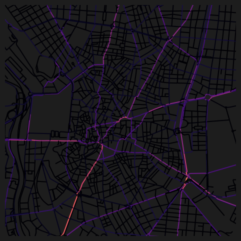

Tolerance for near-shortest paths

The tolerance parameter allows betweenness to count paths that are within a given percentage of the shortest path. For example, tolerance=2.0 treats paths within 2% of the shortest as equally valid. This can produce more realistic betweenness distributions by accounting for near-optimal route choices.

distances = [5000]
nodes_gdf = networks.node_centrality_shortest(
    network_structure=network_structure,
    nodes_gdf=nodes_gdf,
    distances=distances,
    sample=True,
    tolerance=0.5,  # percent <= 1% recommended
)
nodes_gdf.columns

INFO:cityseer.metrics.networks:Computing node centrality (shortest).
WARNING:cityseer.metrics.networks:Sampling is experimental: API and behaviour may change in future releases.
INFO:cityseer.metrics.networks:  Sampled 5000m: p=59%

Index(['ns_node_idx', 'x', 'y', 'z', 'live', 'weight', 'primal_edge',
       'primal_edge_node_a', 'primal_edge_node_b', 'primal_edge_idx',
       'dual_node', 'cc_beta_500', 'cc_beta_2000', 'cc_cycles_500',
       'cc_cycles_2000', 'cc_density_500', 'cc_density_2000', 'cc_farness_500',
       'cc_farness_2000', 'cc_harmonic_500', 'cc_harmonic_2000',
       'cc_hillier_500', 'cc_hillier_2000', 'cc_betweenness_500',
       'cc_betweenness_2000', 'cc_betweenness_beta_500',
       'cc_betweenness_beta_2000', 'cc_beta_1200', 'cc_cycles_1200',
       'cc_density_1200', 'cc_farness_1200', 'cc_harmonic_1200',
       'cc_hillier_1200', 'cc_betweenness_1200', 'cc_betweenness_beta_1200',
       'cc_beta_400', 'cc_cycles_400', 'cc_density_400', 'cc_farness_400',
       'cc_harmonic_400', 'cc_hillier_400', 'cc_betweenness_400',
       'cc_betweenness_beta_400', 'cc_beta_10000', 'cc_cycles_10000',
       'cc_density_10000', 'cc_farness_10000', 'cc_harmonic_10000',
       'cc_hillier_10000', 'cc_betweenness_10000', 'cc_betweenness_beta_10000',
       'cc_beta_5000', 'cc_cycles_5000', 'cc_density_5000', 'cc_farness_5000',
       'cc_harmonic_5000', 'cc_hillier_5000', 'cc_betweenness_5000',
       'cc_betweenness_beta_5000'],
      dtype='object')

fig, ax = plt.subplots(1, 1, figsize=(8, 6), facecolor="#1d1d1d")
nodes_gdf.plot(
    column="cc_betweenness_5000",
    cmap="magma",
    legend=False,
    ax=ax,
)
ax.set_xlim(438500, 438500 + 3500)
ax.set_ylim(4472500, 4472500 + 3500)
ax.axis(False)

(np.float64(438500.0),
 np.float64(442000.0),
 np.float64(4472500.0),
 np.float64(4476000.0))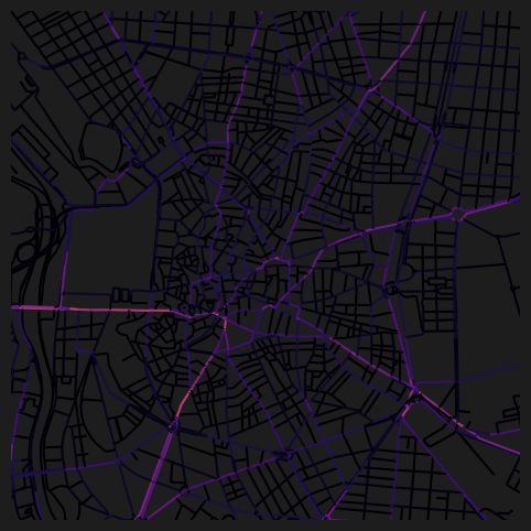

Summary

This notebook demonstrated how to calculate metric (shortest-path) centralities from a geopandas GeoDataFrame. It covered setting live nodes from a boundary to prevent edge rolloff, computing centralities at multiple distance thresholds, using minutes and betas as alternative ways to specify thresholds, and using the sample parameter for efficient computation at larger distances. It also showed the tolerance parameter for near-shortest path betweenness.

Next steps:

To calculate angular (simplest-path) centralities instead, see Angular Centrality.
To calculate centralities directly from OpenStreetMap data, see OSM Centrality.
To compute accessibility or mixed-use metrics over the same network, see the Accessibility recipes.