import matplotlib.pyplot as pltimport momepyimport pandas as pdimport seaborn as snsfrom cityseer.metrics import layersfrom cityseer.tools import graphs, iofrom matplotlib import colorsfrom osmnx import features
/Users/gareth/dev/benchmark-urbanism/cityseer-examples/.venv/lib/python3.12/site-packages/tqdm/auto.py:21: TqdmWarning: IProgress not found. Please update jupyter and ipywidgets. See https://ipywidgets.readthedocs.io/en/stable/user_install.html
  from .autonotebook import tqdm as notebook_tqdm
To start, follow the same approach as shown in the network examples to create the network.
lng, lat =-0.13396079424572427, 51.51371088849723buffer=1500poly_wgs, epsg_code = io.buffered_point_poly(lng, lat, buffer)G = io.osm_graph_from_poly(poly_wgs)G = graphs.nx_decompose(G, 50)G_dual = graphs.nx_to_dual(G)nodes_gdf, _edges_gdf, network_structure = io.network_structure_from_nx(G_dual)
INFO:cityseer.tools.graphs:Generating interpolated edge geometries.
WARNING:cityseer.tools.util:The to_crs_code parameter 4326 is not a projected CRS
INFO:cityseer.tools.io:Converting networkX graph to CRS code 32630.
WARNING:cityseer.tools.util:The to_crs_code parameter 4326 is not a projected CRS
INFO:cityseer.tools.io:Processing node x, y coordinates.
INFO:cityseer.tools.io:Processing edge geom coordinates, if present.
INFO:cityseer.tools.graphs:Removing filler nodes.
INFO:cityseer.tools.util:Creating edges STR tree.
INFO:cityseer.tools.graphs:Removing filler nodes.
INFO:cityseer.tools.graphs:Removing dangling nodes.
INFO:cityseer.tools.graphs:Removing filler nodes.
INFO:cityseer.tools.util:Creating edges STR tree.
INFO:cityseer.tools.graphs:Splitting opposing edges.
INFO:cityseer.tools.graphs:Squashing opposing nodes
INFO:cityseer.tools.graphs:Merging parallel edges within buffer of 25.
INFO:cityseer.tools.util:Creating edges STR tree.
INFO:cityseer.tools.graphs:Splitting opposing edges.
INFO:cityseer.tools.graphs:Squashing opposing nodes
INFO:cityseer.tools.graphs:Merging parallel edges within buffer of 25.
INFO:cityseer.tools.util:Creating edges STR tree.
INFO:cityseer.tools.graphs:Splitting opposing edges.
INFO:cityseer.tools.graphs:Squashing opposing nodes
INFO:cityseer.tools.graphs:Merging parallel edges within buffer of 25.
INFO:cityseer.tools.util:Creating edges STR tree.
INFO:cityseer.tools.graphs:Splitting opposing edges.
INFO:cityseer.tools.graphs:Squashing opposing nodes
INFO:cityseer.tools.graphs:Merging parallel edges within buffer of 25.
INFO:cityseer.tools.util:Creating nodes STR tree
INFO:cityseer.tools.graphs:Consolidating nodes.
INFO:cityseer.tools.graphs:Merging parallel edges within buffer of 25.
INFO:cityseer.tools.graphs:Removing filler nodes.
INFO:cityseer.tools.util:Creating nodes STR tree
INFO:cityseer.tools.graphs:Consolidating nodes.
INFO:cityseer.tools.graphs:Merging parallel edges within buffer of 25.
INFO:cityseer.tools.graphs:Removing filler nodes.
INFO:cityseer.tools.util:Creating nodes STR tree
INFO:cityseer.tools.graphs:Consolidating nodes.
INFO:cityseer.tools.graphs:Merging parallel edges within buffer of 25.
INFO:cityseer.tools.graphs:Removing filler nodes.
INFO:cityseer.tools.util:Creating nodes STR tree
INFO:cityseer.tools.graphs:Consolidating nodes.
INFO:cityseer.tools.graphs:Merging parallel edges within buffer of 25.
INFO:cityseer.tools.graphs:Removing filler nodes.
INFO:cityseer.tools.util:Creating nodes STR tree
INFO:cityseer.tools.util:Creating edges STR tree.
INFO:cityseer.tools.graphs:Snapping gapped endings.
INFO:cityseer.tools.util:Creating edges STR tree.
INFO:cityseer.tools.graphs:Splitting opposing edges.
INFO:cityseer.tools.graphs:Merging parallel edges within buffer of 25.
INFO:cityseer.tools.graphs:Removing dangling nodes.
INFO:cityseer.tools.graphs:Removing filler nodes.
INFO:cityseer.tools.util:Creating edges STR tree.
INFO:cityseer.tools.graphs:Splitting opposing edges.
INFO:cityseer.tools.graphs:Squashing opposing nodes
INFO:cityseer.tools.graphs:Merging parallel edges within buffer of 25.
INFO:cityseer.tools.util:Creating nodes STR tree
INFO:cityseer.tools.graphs:Consolidating nodes.
INFO:cityseer.tools.graphs:Merging parallel edges within buffer of 25.
INFO:cityseer.tools.graphs:Removing filler nodes.
INFO:cityseer.tools.graphs:Merging parallel edges within buffer of 50.
INFO:cityseer.tools.graphs:Ironing edges.
INFO:cityseer.tools.graphs:Merging parallel edges within buffer of 1.
INFO:cityseer.tools.graphs:Removing dangling nodes.
INFO:cityseer.tools.graphs:Removing filler nodes.
INFO:cityseer.tools.graphs:Decomposing graph to maximum edge lengths of 50.
INFO:cityseer.tools.graphs:Converting graph to dual.
INFO:cityseer.tools.graphs:Preparing dual nodes
INFO:cityseer.tools.graphs:Preparing dual edges (splitting and welding geoms)
INFO:cityseer.tools.io:Preparing node and edge arrays from networkX graph.
INFO:cityseer.graph:Edge R-tree built successfully with 9061 items.
Prepare the buildings GeoDataFrame by downloading the data from OpenStreetMap. The osmnxfeatures_from_polygon works well for this purpose. In this instance, we are specifically targeting features that are labelled as an building.
It is important to convert the derivative GeoDataFrame to the same CRS as the network.
Some preparatory data cleaning is typically necessary. This example extracts the particular rows and columns of interest for the subsequent steps of analysis.
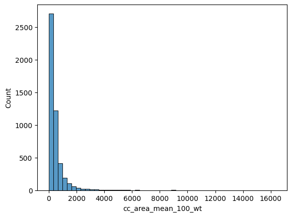
Use the layers.compute_stats method to compute statistics for numeric columns in the GeoDataFrame. These are specified with the stats_column_labels argument. These statistics are computed over the network using network distances. In the case of weighted variances, the contribution of any particular point is weighted by the distance from the point of measure.
INFO:cityseer.metrics.layers:Computing statistics.
INFO:cityseer.metrics.layers:Assigning data to network.
INFO:cityseer.data:Assigning 9768 data entries to network nodes (max_dist: 100).
INFO:cityseer.data:Finished assigning data. 90508 assignments added to 4910 nodes.
INFO:cityseer.config:Metrics computed for:
INFO:cityseer.config:Distance: 100m, Beta: 0.04, Walking Time: 1.25 minutes.
INFO:cityseer.config:Distance: 200m, Beta: 0.02, Walking Time: 2.5 minutes.
This will generate a set of columns containing count, sum, min, max, mean, and var, in unweighted nw and weighted wt versions (where applicable) for each of the input distance thresholds.
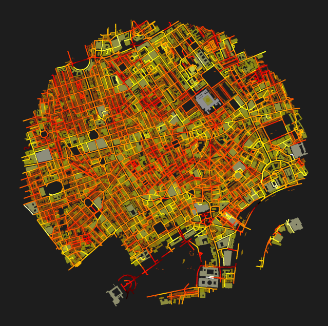
This notebook demonstrated how to compute network-distance-weighted building statistics from OpenStreetMap data for London, using osmnx to fetch building footprints and momepy to derive morphological attributes (area, perimeter, compactness, orientation, shape index). The compute_stats function aggregates these numeric attributes over the network at specified distance thresholds.
Next steps: For visual enclosure metrics, see Visibility.